The Disk
The disk is normally treated as infinitely thin and defined by an inner boundary and an outer boundary. It assumed to be in Keplerian rotation about the central object in the system. The temperature distribution of the disk is normally assumed to be that of a standard Shakura-Sunyaev disk, with a hard boundary at its inner edge. Options are provided for reading in a non-standard temperature distribution.
An option is provide for a vertically extended disk, whose thickness increases as with distance from the central object object.
The parameters involved in describing a flat disk are:
Disk.type(none,flat,vertically.extended)                 flat
Disk.radiation(yes,no)                          yes
Disk.rad_type_to_make_wind(bb,models,mod_bb)                   bb
Disk.temperature.profile(standard,readin)             standard
Disk.mdot(msol/yr)                         5
Disk.radmax(cm)                            1e17
Colour Correction (mod_bb)
A simple form of the disc colour correction is available in the code, accessible via the Disk.rad_type_to_make_wind keyword. The colour correction factor, \(f_{\rm col}\), is defined such that
This correction is designed to approximate the effect of radiative transfer in the disc atmosphere. We adopt the form given by Done et al. 2012, in which \(f_{\rm col}=1\) for \(T<3\times10^4~{\rm K}\), and for \(T>3\times10^4~{\rm K}\)
Vertically Extended disk (Details)
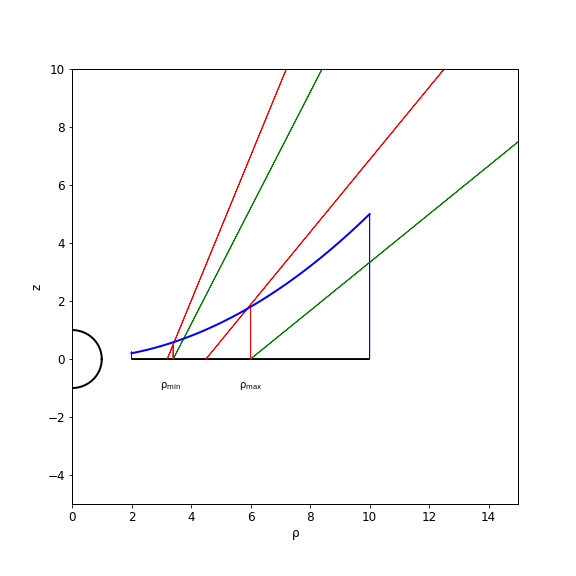
The figure above explains the basics issues associated with a vertically extended disk. The wind emerges from the actual disk between \(\rho_{min}\) and \(\rho_{max}\).
In defining a vertically extended disk in the context of parameterized models, such as KWD of SV, one needs to decide how to tranlated values from a parameterized wind on a flat disk to a parameterized wind on verticallye extended disk. The choices we have made are (intended to be) as follows:
The temperature and luminosity of a vertically extended disk are given by the distance from the central object in the disk plane.
The density at the base of the wind is defined as the same as the flat disk that underlies it.
The poloidal (and rotational) velocity at the footpoint is the poloidal velocity along the streamline, starting with \(v_{}\) at the actual surface of the disk.
For the SV model, the streamline direction and velocity are determined by the distance from the central object along the disk plane. This is not the same as one would obtain by projecting the streamline back to the disk plane.
For the KWD disk, stream line directions that reflect the focus position and the poloidal velocity ate taken from that expected by projecting the stream line back to the disk plane.
(Note that the in the KWD case, there is a slight inconsistency/inaccuracy in calculating desired mass loss rates, because the mass loss rate is calculate as if the disk were flat, but the stream line directions are not exactly the same as due to the vertical extension of the disk. There are also issues more generally because we do not take into account the fact that the disk area of a vertically extended disk is not exactly the same as that of a flat disk.)
Non-Standard Temperature Profile
If desired the user can read the temperature profile for the disk from a file. Each line in the file should consist of a radius (in cm) and a temperature (in K), and optionally a value of \(\log g\). The values separated by whitespace (in the first two columns). The values are assumed to be entered in a logical order, that is in ascending values of radius. Lines such as comments or header names of an astropy table, will be ignored.
The \(\log g\) value is not required to generate BB spectra, but is required if the spectrum from the disk is to be generated from a two-dimensional grid of models, usually a set of spectra generated to represent the spectra from a set of stellar atmospheres calculations.
With this option, the radius of the disk will be set to the maximum radius (the last value of r) in the file.