Ionization Spectral Modelling

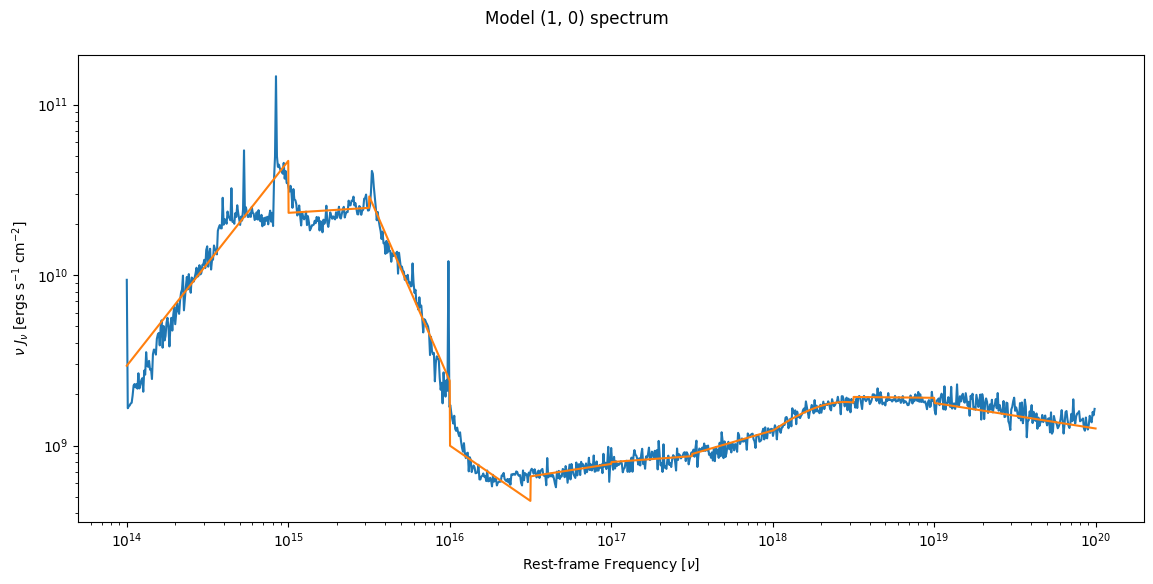
One important aspect of SIROCCO is that, when using one of the rate matrix options for the ionization treatment of simple atoms, a model for the mean intensity is required. Through the Wind.ionization keyword, the user has the option to model the mean intensity either as a dilute blackbody (matrix_bb: \(J_\nu = W B_\nu(T_r)\)) or following the procedure described by Higginbottom+ 2013 (matrix_pow). In the latter case, we construct a model for the mean intensity by splitting the entire frequency range into a series of coarse bands, where the bands are usually explicitly tied to photon generation (but with a minimum of seven frequency bands for the spectral model).

It is important to ensure the spectral model reasonably characterises the in cell spectrum and that the banding strategy chosen is sufficient. You may need to adjust the banding based on running these diagnostics, particular if there are too few bands for the complexity of the spectrum. Please see the banding page, as well as these github issues.

This notebook shows you how to use PySi to look at the in cell spectrum for a given cell, as well as the spectral model in that cell. This code can then be adjusted to look at cell spectra and models for an entire simulation. Before running the below code, you must have run

windsave2table -xall run_name

On your simulation named run_name.

Please note that macro-atoms always have their level populations and ion fractions obtained self-consistently from MC estimators following Lucy (2003) (see e.g., Matthews thesis).

import matplotlib.pyplot as plt
import numpy as np
import pysi
from pysi.wind import Wind
root = "run128"
directory = "agn_test/"
wind = Wind(root = root, directory = directory)

i, j = wind.get_ij_from_elem_number(100) # gets the i,j coordinate for wind cell 100
fig, ax = wind.plot_cell_spectrum(i,j)
_ = wind.plot_cell_model(i,j, fig=fig, ax=ax)

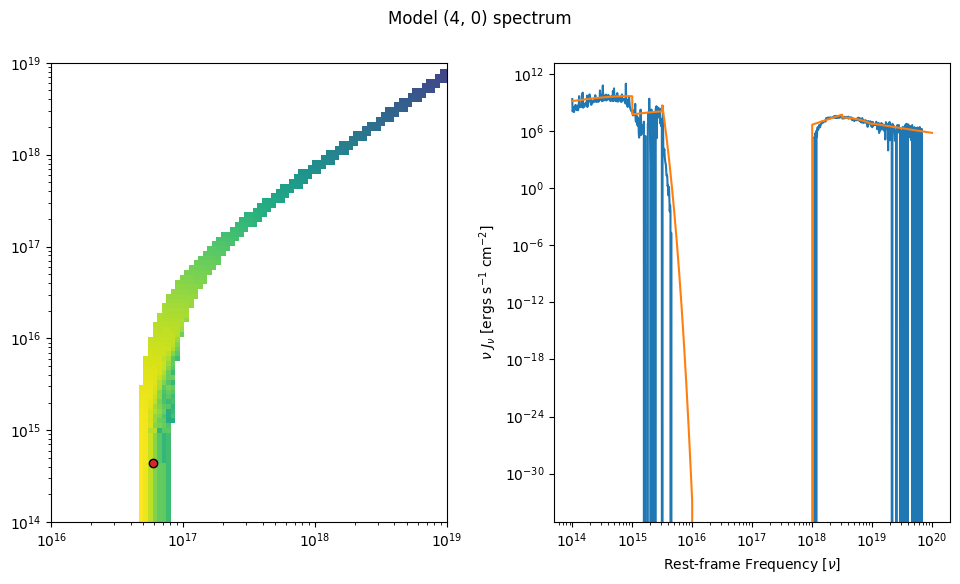
The following function will make a plot that shows you what is happening under the hood (i.e. which variables contain the information) and also where the cell is in the wind.

def cell_spectrum_plot(nwind):
    i, j = wind.get_ij_from_elem_number(nwind)

    if wind["inwind"][i,j] < 0:
        print ("Cell {} is not in wind".format(nwind))
        return None, None

    fig, ax = plt.subplots(figsize = (10,6), nrows = 1, ncols = 2)
    ax[0].pcolormesh(wind["x"], wind["z"], np.log10(wind["ne"]), cmap="viridis")
    ax[0].scatter(wind["xcen"][i,j], wind["zcen"][i,j], c="C3", ec="k")
    ax[0].loglog()
    ax[0].set_xlim(1e16,1e19)
    ax[0].set_ylim(1e14,1e19)

    wind.plot_cell_spectrum(i,j, fig=fig, ax=ax[1])
    wind.plot_cell_model(i,j, fig=fig, ax=ax[1])
    # the below is a way to do this manually
    # ax[1].plot(wind["spec_freq"][i,j], wind["spec_flux"][i,j])
    # ax[1].plot(wind["model_freq"][i,j], wind["model_flux"][i,j])
    # ax[1].loglog()
    return (fig, ax)

cell_spectrum_plot(2)
_ = cell_spectrum_plot(400)

Cell 2 is not in wind

/Users/matthewsj/.mpi_temp/ipykernel_95633/2141820871.py:9: RuntimeWarning: divide by zero encountered in log10
  ax[0].pcolormesh(wind["x"], wind["z"], np.log10(wind["ne"]), cmap="viridis")

Note the use of the inwind variable to avoid the cells outside the wind. To loop over the wind domain, you can embed the above function in a for loop over the total number of wind cells obtained from. Here’s a function that, combined with the above function, would do that and save the above plot for every cell in the wind for a given root like run128.

def all_cell_spectra(run_name="run128", directory ="agn_test/"):
    wind = Wind(root = root, directory = directory)
    for n in range(wind.n_cells):
        fig, ax = cell_spectrum_plot(n)
        if fig is not None:fig.savefig("incell_{}_{}.png".format(run_name, n))