Plotting Wind Properties

As described under Models, SIROCCO saves wind properties in binary wind_save files. This notebook explains how to read and plot wind variables for the cv_standard file found in the examples. Before running the python commands, you need to run the model from the command line. I suggest running the following commands, after you have compiled python:

mkdir cv_test
cd cv_test
cp $SIROCCO/examples/basic/cv_standard.pf .
sirocco cv_standard </code>

The model will take about 5 minutes to run on a single core. It will not converge, but will give us a model to use as an example. You should then run windsave2table on the output

windsave2table cv_standard

which will create a series of ascii files containing key variables in the wind cells. We will use these ascii files for our plots.

Making wind plots using PySi

We will start by demonstrating how to use PySi to plot data from the wind files. In particular we will plot some key variables in the wind, followed by some ion fractions.

PySi works by setting up a Wind class which reads in and stores all the useful data and attributes from the model. This class can be used to inspect data or to plot it directly.

[1]:

import matplotlib.pyplot as plt
import numpy as np
import pysi
from pysi.wind import Wind
root = "cv_standard"
directory = "cv_test/"
wind = Wind(root = root, directory = directory)

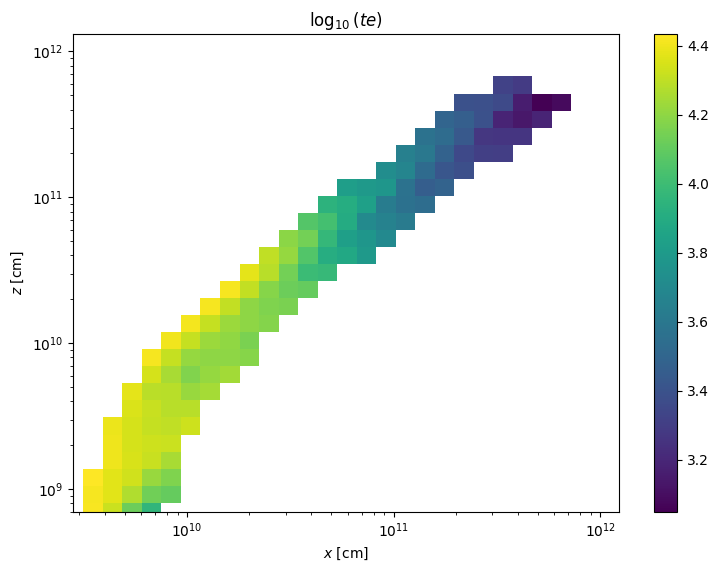
The data can be plotted easily using the plot_parameter method. This method returns Figure and Axes objects so the plot can be modified easily.

[2]:

fig, ax = wind.plot_parameter("t_e")

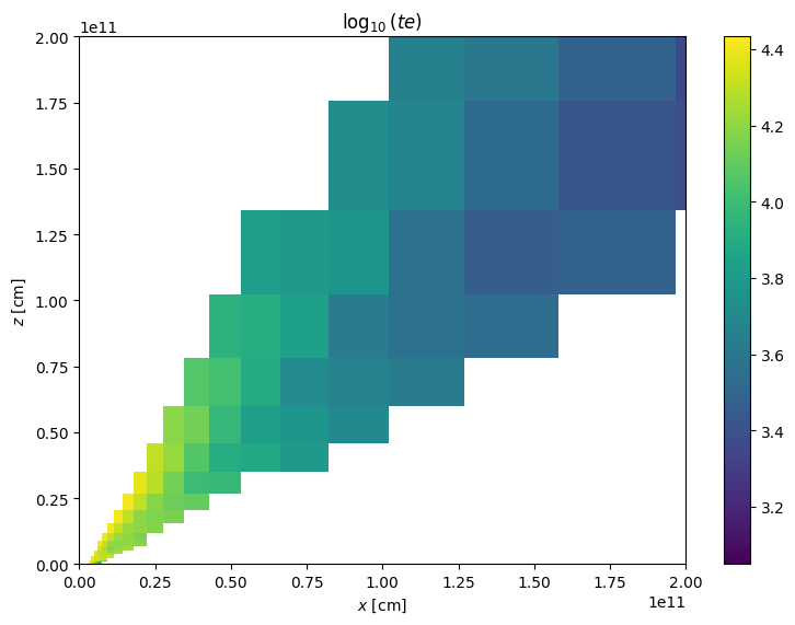
[3]:

plot = wind.plot_parameter("t_e", "linlin")
plt.xlim(0,2e11)
_ = plt.ylim(0,2e11)

The get_windsave_descriptions method in the wind class comes provides a handy guide to the main columns in the .master.txt file, which can be plotted using the above methods, or accessed directly as, e.g., wind["ne"]

[4]:

print (wind.get_windsave_descriptions())

x          --  left-hand lower cell corner x-coordinate, cm
z          --  left-hand lower cell corner z-coordinate, cm
xcen       --  cell centre x-coordinate, cm
zcen       --  cell centre z-coordinate, cm
i          --  cell index (column)
j          --  cell index (row)
inwind     --  is the cell in wind (0), partially in wind (1) or out of wind (<0)
converge   --  how many convergence criteria is the cell failing?
v_x        --  x-velocity, cm/s
v_y        --  y-velocity, cm/s
v_z        --  z-velocity, cm/s
vol        --  volume in cm^3
rho        --  density in g/cm^3
ne         --  electron density in cm^-3
t_e        --  electron temperature in K
t_r        --  radiation temperature in K
h1         --  H1 ion fraction
he2        --  He2 ion fraction
c4         --  C4 ion fraction
n5         --  N5 ion fraction
o6         --  O6 ion fraction
dmo_dt_x   --  momentum rate, x-direction
dmo_dt_y   --  momentum rate, y-direction
dmo_dt_z   --  momentum rate, z-direction
ip         --  U ionization parameter
xi         --  xi ionization parameter
ntot       --  total photons passing through cell
nrad       --  total wind photons produced in cell
nioniz     --  total ionizing photons passing through cell
None

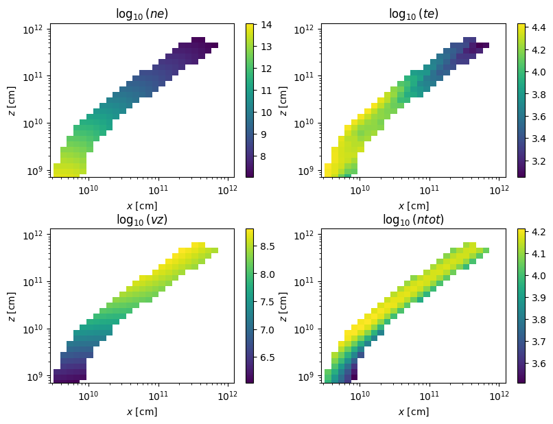
We can also use the multiplot command to generate multiple plots for specified wind parameters. This method creates subplots to visualize the specified wind parameters using either 1D or 2D representation based on the coordinate system.

[5]:

fig, ax = wind.multiplot( ("ne", "t_e", "v_z", "ntot") , "loglog", nrows = 2, ncols = 2)
fig.tight_layout(pad=0.05)

We can also check all the possible things to plot, some of which are intuitive and some of which aren’t!

[6]:

print (wind.things_read_in)

dict_keys(['x', 'z', 'xcen', 'zcen', 'i', 'j', 'inwind', 'converge', 'v_x', 'v_y', 'v_z', 'vol', 'rho', 'ne', 't_e', 't_r', 'h1', 'he2', 'c4', 'n5', 'o6', 'dmo_dt_x', 'dmo_dt_y', 'dmo_dt_z', 'ip', 'xi', 'ntot', 'nrad', 'nioniz', 'w', 'ave_freq', 'J', 'J_direct', 'J_scatt', 'lum_tot', 'heat_tot', 'heat_comp', 'heat_line', 'heat_ff', 'heat_phot', 'heat_auge', 'cool_tot', 'cool_comp', 'lum_lines', 'cool_dr', 'lum_ff', 'lum_rr', 'cool_rr', 'cool_adia', 'heat_shoc', 'ht_ln_mac', 'ht_ph_mac', 'dv_x_dx', 'dv_y_dx', 'dv_z_dx', 'dv_x_dy', 'dv_y_dy', 'dv_z_dy', 'dv_x_dz', 'dv_y_dz', 'dv_z_dz', 'div_v', 'dvds_max', 'gamma', 'dfudge', 't_e_old', 'dt_e', 'dt_e_old', 't_r_old', 'heat_tot_', 'gain', 'macro_bf_', 'H_i01_frac', 'H_i02_frac', 'He_i01_frac', 'He_i02_frac', 'He_i03_frac', 'C_i01_frac', 'C_i02_frac', 'C_i03_frac', 'C_i04_frac', 'C_i05_frac', 'C_i06_frac', 'C_i07_frac', 'N_i01_frac', 'N_i02_frac', 'N_i03_frac', 'N_i04_frac', 'N_i05_frac', 'N_i06_frac', 'N_i07_frac', 'N_i08_frac', 'O_i01_frac', 'O_i02_frac', 'O_i03_frac', 'O_i04_frac', 'O_i05_frac', 'O_i06_frac', 'O_i07_frac', 'O_i08_frac', 'O_i09_frac', 'Na_i01_frac', 'Na_i02_frac', 'Na_i03_frac', 'Na_i04_frac', 'Na_i05_frac', 'Na_i06_frac', 'Na_i07_frac', 'Na_i08_frac', 'Na_i09_frac', 'Na_i10_frac', 'Na_i11_frac', 'Na_i12_frac', 'Si_i01_frac', 'Si_i02_frac', 'Si_i03_frac', 'Si_i04_frac', 'Si_i05_frac', 'Si_i06_frac', 'Si_i07_frac', 'Si_i08_frac', 'Si_i09_frac', 'Si_i10_frac', 'Si_i11_frac', 'Si_i12_frac', 'Si_i13_frac', 'Si_i14_frac', 'Si_i15_frac', 'Ca_i01_frac', 'Ca_i02_frac', 'Ca_i03_frac', 'Ca_i04_frac', 'Ca_i05_frac', 'Ca_i06_frac', 'Ca_i07_frac', 'Ca_i08_frac', 'Ca_i09_frac', 'Ca_i10_frac', 'Ca_i11_frac', 'Ca_i12_frac', 'Ca_i13_frac', 'Ca_i14_frac', 'Ca_i15_frac', 'Ca_i16_frac', 'Ca_i17_frac', 'Ca_i18_frac', 'Ca_i19_frac', 'Ca_i20_frac', 'Ca_i21_frac', 'Fe_i01_frac', 'Fe_i02_frac', 'Fe_i03_frac', 'Fe_i04_frac', 'Fe_i05_frac', 'Fe_i06_frac', 'Fe_i07_frac', 'Fe_i08_frac', 'Fe_i09_frac', 'Fe_i10_frac', 'Fe_i11_frac', 'Fe_i12_frac', 'Fe_i13_frac', 'Fe_i14_frac', 'Fe_i15_frac', 'Fe_i16_frac', 'Fe_i17_frac', 'Fe_i18_frac', 'Fe_i19_frac', 'Fe_i20_frac', 'Fe_i21_frac', 'Fe_i22_frac', 'Fe_i23_frac', 'Fe_i24_frac', 'Fe_i25_frac', 'Fe_i26_frac', 'Fe_i27_frac', 'spec_freq', 'spec_flux', 'model_freq', 'model_flux', 'v_l', 'v_rot', 'v_r'])

Plotting ions using PySi

PySi also allows one to plot ion fractions or densities (fractions by default), which are accessed through strings like Fe_i01_frac, using astronomical notation for the ion stage. An example multiplot of the first six ionic stages of Carbon would be as follows.

[7]:

ions_to_plot = ["C_i{:02d}_frac".format(i+1) for i in range(6)]
fig, ax = wind.multiplot(ions_to_plot, "loglog", nrows = 3, ncols = 2, figsize=(8,10))

All the ions in the simulation can be viewed using the ions_read_in list.

[8]:

print (wind.ions_read_in)

['H_i01_frac', 'H_i02_frac', 'He_i01_frac', 'He_i02_frac', 'He_i03_frac', 'C_i01_frac', 'C_i02_frac', 'C_i03_frac', 'C_i04_frac', 'C_i05_frac', 'C_i06_frac', 'C_i07_frac', 'N_i01_frac', 'N_i02_frac', 'N_i03_frac', 'N_i04_frac', 'N_i05_frac', 'N_i06_frac', 'N_i07_frac', 'N_i08_frac', 'O_i01_frac', 'O_i02_frac', 'O_i03_frac', 'O_i04_frac', 'O_i05_frac', 'O_i06_frac', 'O_i07_frac', 'O_i08_frac', 'O_i09_frac', 'Na_i01_frac', 'Na_i02_frac', 'Na_i03_frac', 'Na_i04_frac', 'Na_i05_frac', 'Na_i06_frac', 'Na_i07_frac', 'Na_i08_frac', 'Na_i09_frac', 'Na_i10_frac', 'Na_i11_frac', 'Na_i12_frac', 'Si_i01_frac', 'Si_i02_frac', 'Si_i03_frac', 'Si_i04_frac', 'Si_i05_frac', 'Si_i06_frac', 'Si_i07_frac', 'Si_i08_frac', 'Si_i09_frac', 'Si_i10_frac', 'Si_i11_frac', 'Si_i12_frac', 'Si_i13_frac', 'Si_i14_frac', 'Si_i15_frac', 'Ca_i01_frac', 'Ca_i02_frac', 'Ca_i03_frac', 'Ca_i04_frac', 'Ca_i05_frac', 'Ca_i06_frac', 'Ca_i07_frac', 'Ca_i08_frac', 'Ca_i09_frac', 'Ca_i10_frac', 'Ca_i11_frac', 'Ca_i12_frac', 'Ca_i13_frac', 'Ca_i14_frac', 'Ca_i15_frac', 'Ca_i16_frac', 'Ca_i17_frac', 'Ca_i18_frac', 'Ca_i19_frac', 'Ca_i20_frac', 'Ca_i21_frac', 'Fe_i01_frac', 'Fe_i02_frac', 'Fe_i03_frac', 'Fe_i04_frac', 'Fe_i05_frac', 'Fe_i06_frac', 'Fe_i07_frac', 'Fe_i08_frac', 'Fe_i09_frac', 'Fe_i10_frac', 'Fe_i11_frac', 'Fe_i12_frac', 'Fe_i13_frac', 'Fe_i14_frac', 'Fe_i15_frac', 'Fe_i16_frac', 'Fe_i17_frac', 'Fe_i18_frac', 'Fe_i19_frac', 'Fe_i20_frac', 'Fe_i21_frac', 'Fe_i22_frac', 'Fe_i23_frac', 'Fe_i24_frac', 'Fe_i25_frac', 'Fe_i26_frac', 'Fe_i27_frac']

More direct data access

We recommend using PySi where possible. You may, however, wish to get more direct access to the data, which can be done easily by reading in the cv_standard.master.txt file, for example using astropy. In the next code block, we read in the data file and print out the columns.

[9]:

import matplotlib.pyplot as plt
import astropy.io.ascii as io

fname = f"{directory}{root}.master.txt"
data = io.read(fname)

print (data.colnames)

['x', 'z', 'xcen', 'zcen', 'i', 'j', 'inwind', 'converge', 'v_x', 'v_y', 'v_z', 'vol', 'rho', 'ne', 't_e', 't_r', 'h1', 'he2', 'c4', 'n5', 'o6', 'dmo_dt_x', 'dmo_dt_y', 'dmo_dt_z', 'ip', 'xi', 'ntot', 'nrad', 'nioniz']

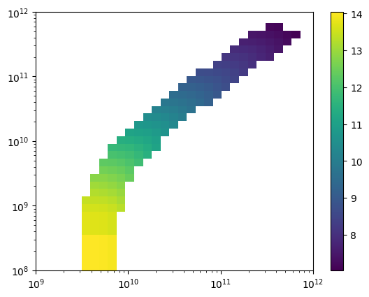
py_plot_util, found in the $SIROCCO/py_progs/ directory, also contains some routines for reshaping and masking arrays and so on. One of the most useful for plotting is the wind_to_masked function which turns the raw 1D flattened data into a masked 2D array with the right shape which can be easily used with pcolormesh and so on. Here’s an example plot of the electron density in the model.

[10]:

import py_plot_util as util
x, z, ne, inwind = util.wind_to_masked(data, value_string="ne", return_inwind=True)
plt.pcolormesh(x,z, np.log10(ne))
plt.loglog()
plt.xlim(1e9,1e12)
plt.ylim(1e8,1e12)
cbar = plt.colorbar()

/Users/matthewsj/.mpi_temp/ipykernel_40675/3684827325.py:3: RuntimeWarning: divide by zero encountered in log10
  plt.pcolormesh(x,z, np.log10(ne))

This procedure can be used to plot any of the variables in the masterfile and is a good starting point for delving into the properties of the wind if not using PySi.

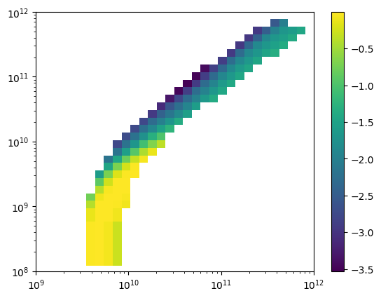
Ion populations outputted from windsave2table are stored in files like cv_standard.C.frac.txt, where the letter before frac denotes the element. Plots of the C III ion fraction can thus be made through commands like the following, where strings like i05 index the ion for each file.

[11]:

carbon_ion = io.read("cv_test/cv_standard.C.frac.txt")
x, z, c3_frac, inwind = util.wind_to_masked(carbon_ion, value_string="i03", return_inwind=True)
plt.pcolormesh(x,z, np.log10(c3_frac))
plt.loglog()
plt.xlim(1e9,1e12)
plt.ylim(1e8,1e12)
cbar = plt.colorbar()

/Users/matthewsj/.mpi_temp/ipykernel_40675/4163463376.py:3: RuntimeWarning: divide by zero encountered in log10
  plt.pcolormesh(x,z, np.log10(c3_frac))

Make A Basic Quick Look Wind Plot

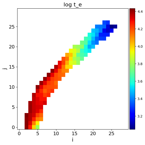
The simplest way to make a quick look plot of the electron temperature is using the plot_wind.py routine in $SIROCCO/py_progs. In this example, I will assume py_progs has been added to $PATH and to $PYTHONPATH. plot_wind.py can be run from the command line using

plot_wind.py cv_standard t_e

where the second argument is the variable to plot. Alternatively, it can be run from within a python script by doing (where we are now assuming you are running this code from one directory above cv_test):

[12]:

import matplotlib.pyplot as plt
import numpy as np
import plot_wind
fname = "cv_test/cv_standard.master.txt"
plot_wind.doit(fname, var="t_e")

[12]:

'cv_test/cv_standard_log_t_e.png'